Live Variable Analysis

This implementation, available at Github, leverages a data flow analysis algorithm to trace the variables throughout the program. The control flow and use of variables are considered in the analysis process, which takes place on the intermediate representation of the program represented as a control flow graph.

The algorithm employed is based on the iterative data flow analysis method, where multiple passes are made over the program until the results converge to a stable solution. The implementation was written in Haskell and uses a map structure to store the live variables at each point in the program.

Expressions

An arithmetic expression is given by the following syntax: $e ::= n | x | e_1 + e_2 | e_1 - e_2 | e_1 * e_2$

data AExpression
  = Literal Int
  | Variable String
  | Add AExpression AExpression
  | Sub AExpression AExpression
  | Mul AExpression AExpression

For example, the arithmetic expression x + 1 is represented as: Add (E.Variable "x") (E.Literal 1)

On the other hand, a boolean expression is given by the following syntax: $b ::= e_1 \leq e_2 | e_1 = e_2 | b_1 \land b_2$

data BExpression
  = Leq AExpression AExpression
  | Equal AExpression AExpression
  | And BExpression BExpression

For example, the boolean expression x <= 1 is represented as: Leq (E.Variable "x") (E.Literal 1)

Representation of the Control Flow Graph

In this implementation, programs are encoded into a CFG, where the basic blocks are assignments and boolean expressions. Each basic block will contain a unique label. In live variable analysis, the process receives a program’s Control Flow Graph (CFG) and yields, for every block in the CFG, the set of live variables before and after that block.

Here is an example in While:

x := 1
while y > 0 do
    y := y - 1;
    x := 2;

CFG

A Control-Flow Graph (CFG) is a list of blocks. Blocks can be either assignments or conditional. In this implementation, we use the following data structures to represent a CFG:

type CFG = [Block]

data BlockType
  = Skip
  | Assignment String E.AExpression
  | Conditional E.BExpression

For instance, the assignment x = 1 can be represented as: Assignment (Add (E.Variable "x") (E.Literal 1)

A block from the CFG is represented as a record than contains a block (block type), an outLink (exit blocks) and the label. In this implementation, each block is represented according to the following data structure:

data Block = Block
  { block :: BlockType,
    label :: Int,
    outLink :: [Int]
  }

For instance, a block (label “1”) can be represented as the following record:

---------
| x = 1 |---> Block 3
---------
   |
Block 2

The block “1” can be represented as the following record:

Block
  { block: Assignment (Add (E.Variable "x") (E.Literal 1))
    label: 1
    outLink: [2, 3]
  }

Data Flow Equations

For this analysis, we compute the following set of variables:

$LVIn_n$: Live variables at the entry of block n. For this, we use the transfer function:

$VIn_n = (LVOut_n − Kill_n) \cup Gen_n$

where $Gen_n$ are variables that are read in block n, and $Kill_n$: are variables that are written to in block n.
$LVOut_n$: Live variables at the exit of block n. A variable is live at the exit of a block if it is live at the entrance of any of the blocks following it. For instance, the block 1:
```
---------
| x = 1 |---> Block 3
---------
  |
Block 2
```
The $LVout_1$ equation is: $LVOut_1 = LVIn_2 \cup LVIn_3$

Solution of the Equation System

The result of this analysis is a system of equations with unknown variables $(LVOut_1, LVOut_2, …LVIn_n)$. These variables represent the fixed points of $F$, which is defined as the supremum of the ascending Kleene chain. Here, $F$ is the vector:

\[F = \begin{pmatrix} LVout_1 \\ ... \\ LVout_1 \\ LVIn_1 \\ ... \\ LVIn_n \\ \end{pmatrix}\]

The solutions to this system can be found by repeating the following steps until the variables converge to a stable solution:

Solving the data flow equations starts with initializing all LVIn and LVOut to the empty set:
```
LV' = Map (1, LV { LVIn=empty, LVOut=empty })
```
We get the new variable using the previous point:
```
LV'' = getLV LV' ...
```

We repeat (2) until the LV of the previous point is equal to the LV of the current point. This is the solution of our system!

Example

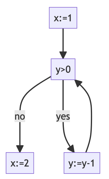
Complete example using the While language:

x := 1
while y > 0 do
    y := y - 1;
    x := 2;

Graphical representation of the control flow graph:

CFG

Representation of the control flow graph in this implementation:

let block1 = G.Assignment "x" (E.Literal 1)
let block2 = G.Conditional (E.Leq (E.Literal 1) (E.Variable "y"))
let block3 = G.Assignment "x" (E.Sub (E.Variable "x") (E.Literal 1))
let block4 = G.Assignment "x" (E.Literal 2)
let graph =
  [
    G.Block {G.label = 1, G.outLink = [2], G.block = block1},
    G.Block {G.label = 2, G.outLink = [3, 4], G.block = block2},
    G.Block {G.label = 3, G.outLink = [2], G.block = block3},
    G.Block {G.label = 4, G.outLink = [], G.block = block4}
  ] :: G.CFG

To run the analysis:

cabal install
cabal run

The Live Variable Analysis result:

LVIn1=["y"] LVOut1=["x","y"]
LVIn2=["x","y"] LVOut2=["x","y"]
LVIn3=["x","y"] LVOut3=["x","y"]
LVIn4=[] LVOut4=[]

References

Lecture notes from “Static Program Analysis and Constraint Solving” at the Universidad Complutense de Madrid, taught by Professor Manuel Montenegro.